
ARIA Brief
How long is a dugong (a sea cow) at an age where none has been observed? In SynthStats, an AI writes the answer as a program that can be run: a statistical model in which lengths scatter around a growth curve.
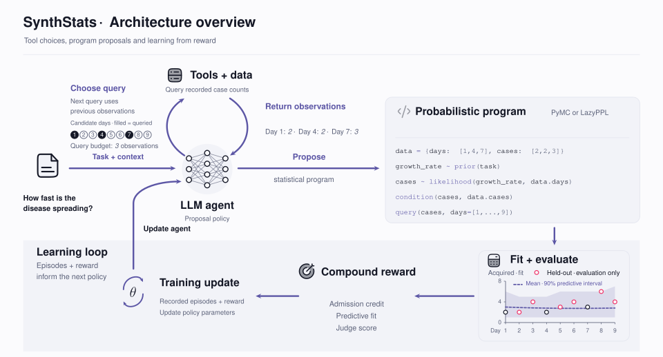
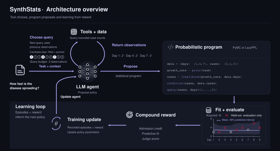
We ask for a program with AI safety in mind: a statistician who opens the dugong program below sees, in a few lines of Python, that it makes length level off with age and uses the same observation-noise scale at every age, and can object to either before relying on its predictions. Before submitting a program, the AI may also request observations and run code of its own.
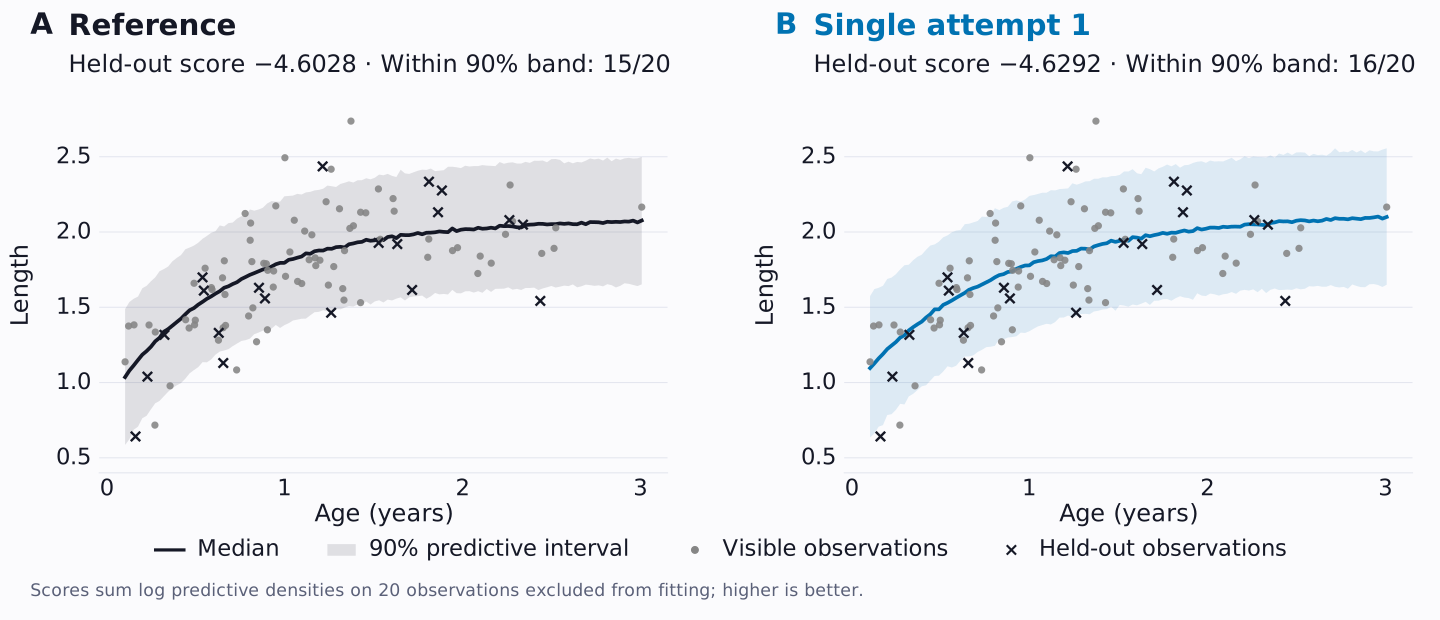
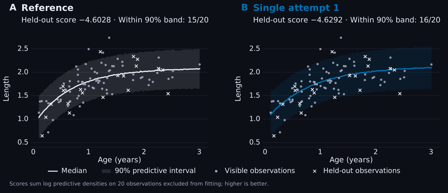
For simulated dugong data, the AI produced an age-length model with the median prediction and 90% predictive interval shown below. The AI here is the prompted language model Qwen3.6-35B-A3B, which wrote the program in a single attempt. We compare the generated program with a reference program written knowing how the simulator generates its data.
| Name | Meaning |
|---|---|
pm | PyMC, a Python library for probability models |
L_inf | Limiting mean length |
k | Sets the growth rate |
t0 | Shifts the curve along the age axis |
sigma | Noise scale around the mean mu |
mu | Mean |
L_inf = pm.HalfNormal("L_inf", sigma=2.0)
k = pm.HalfNormal("k", sigma=1.0)
t0 = pm.Normal("t0", mu=-0.5, sigma=0.5)
mu = L_inf * (1 - pm.math.exp(-k * (age - t0)))
sigma = pm.HalfNormal("sigma", sigma=0.2)
length_obs = pm.Normal("length_obs", mu=mu, sigma=sigma, observed=length)
The generated program infers its Normal noise scale, which the reference fixes at 0.25.
The Monte Carlo standard error (MCSE) measures the error from estimating a score with 200 posterior draws of the fitted model. The 200 draws form ten consecutive batches of 20. Each draw has an influence on the total held-out log score: how much it raises or lowers that total compared with an average draw. We average these influences within each batch. The MCSE is the standard deviation of the ten batch means divided by the square root of ten. A difference between two programs has a combined MCSE: the square root of the sum of the squares of the two MCSEs. The sum treats the two fits as independent. For dugong single attempt 2, which scores 1.4059 above the reference, the MCSE is 0.0190 for the attempt and 0.1031 for the reference, so the combined MCSE is sqrt(0.0190^2 + 0.1031^2) = 0.1048.
| Dugong demonstration | Setting or result |
|---|---|
| Generating language model | Qwen3.6-35B-A3B; single attempt; fixed data |
| Visible / held-out observations | 80 / 20 |
| Generated / reference coverage | 16 / 20; 15 / 20 |
| Generated / reference held-out score ± MCSE | -4.6292 ± 0.0731 / -4.6028 ± 0.1031 |
| Score | Total held-out log predictive density; higher is better |
| Coverage | Held-out observations within central 90% predictive intervals; 5th to 95th percentiles, bounds included |
Predicting infected counts
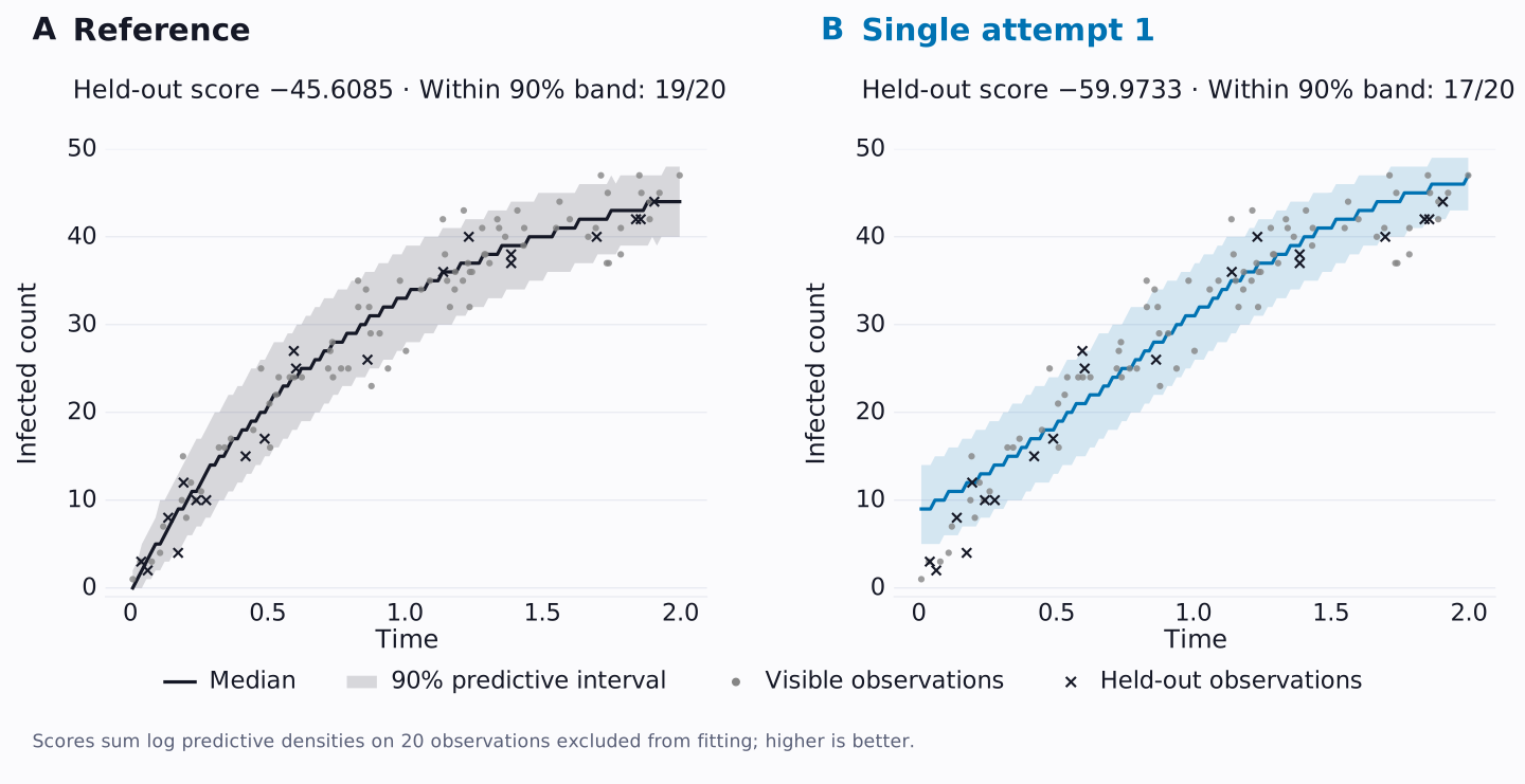
The generated program models counts out of 50 with an S-shaped infection-probability curve. The reference probability approaches one exponentially.
Here N is the population size, alpha and beta set a straight line's intercept and slope, and converting that line to the S-shaped infection-probability curve gives p at each time (the line is the log odds logit_p, and the conversion is the sigmoid).
N = 50  # Total population size
with pm.Model() as pmodel:
    alpha = pm.Normal('alpha', mu=0, sigma=10)
    beta = pm.Normal('beta', mu=0, sigma=10)
    logit_p = alpha + beta * times
    p = pm.math.sigmoid(logit_p)
    infected_observed = pm.Binomial('infected_observed', n=N, p=p, observed=infected_counts)
The last statement connects the model to the data: infected_counts holds the number infected out of N = 50 in each of the 80 visible observations, and the statement models each count as a Binomial draw with 50 individuals and infection probability p at that observation's time.
| Disease-spread demonstration | Setting or result |
|---|---|
| Generating language model | Qwen3.6-35B-A3B; single attempt; fixed data |
| Visible / held-out observations | 80 / 20 |
| Generated / reference coverage | 17 / 20; 19 / 20 |
| Generated / reference held-out score ± MCSE | -59.9733 ± 0.2544 / -45.6085 ± 0.0452 |
One reward for a whole model
At each age, the dugong model above gives a whole distribution of possible lengths, yet in training the AI receives a single reward for such a model. Asked the same question twice, the AI can write two different programs (it can itself be thought of as a distribution over programs), and each program it writes is meant to describe a distribution of observations, which the program may express through unnormalised weights that need not add up to one.
Each attempt at a task, including data requests and any submitted program, is an episode. When the AI submits a program, we check its syntax, safety and model construction against the admission rules. A program that passes is admitted. We fit it and score its predictions on observations withheld from the AI, such as the crosses in the dugong figure. For an admitted program that we can score, utility combines admission credit with a bounded predictive-fit term, q:
| Quantity | Definition |
|---|---|
| Utility of a scorable admitted program | 1.5 + q |
| q | tanh[(ELPD - baseline ELPD) / n]; -1 < q < 1 |
| ELPD | Held-out expected log predictive density: the sum of log predictive densities over the withheld observations |
| baseline ELPD | The task's reference program refitted on its full visible rows with its ordinary predictors replaced by constants computed from those rows alone (a predictor's mean, or its most frequent value if it is categorical) and its structural inputs, such as group membership, offsets and censoring indicators, left at their real values, then scored on its withheld rows with the same constants |
| n | Number of held-out observations |
| Refused or unsubmitted episode | 0 |
The function tanh maps any real number to a value between -1 and 1. The quantity (ELPD - baseline ELPD) / n is the average ELPD difference per held-out observation, and it is 0 when a program's ELPD equals the baseline ELPD, so q = tanh(0) = 0 and the utility is 1.5 + 0 = 1.5. A program that scores above the baseline has a positive q, and one that scores below it has a negative q.
Admission adds more to a program's utility than q can ever add or take away.
In our UAI 2026 paper, Likelihood hacking in probabilistic program synthesis, some of the programs with high rewards made invalid probability claims, in the sense that the probabilities they assigned to all possible datasets did not add up to one. There, we rewarded a language model with the train-split log marginal likelihood that its programs assigned to the data. So our reward has to take normalisation into account, as well as predictive fit.
Paired comparisons of reward training
We trained the larger model, GLM-5.3-Flash, twice with reinforcement learning, starting each time from the untrained model: once with the fit reward, and once with judge-assisted training, in which a language model also grades each program against a rubric. Both rewards combine admission credit and predictive fit, and the judge-assisted arm adds a judge term. For the smaller model, Qwen3.5-0.8B, we first gave the policy a supervised warm start, which trains it to imitate positively rewarded episodes from teacher language models. From that one warm start we ran three arms of reward training, each for eight updates on 220 training packages, and each arm is compared with that same warm start. The first arm applies Subtrajectory Balance (SubTB), an objective computed on segments of the agent's sequence of actions and its rewards; the second applies GRPO, group relative policy optimization, which compares an episode's reward with those of the other episodes on the same task; the third uses the same SubTB objective with the learning rate set to 1e-6, one tenth of the 1e-5 used in the other two arms.
We compare each starting policy with its trained counterpart. For each task, the evaluation package contains its prompt and data, the withheld rows and reference scores. The fit-only and judge-assisted comparisons sampled their untrained episodes separately and used different verifier versions.
| Evaluation and training protocol | Value |
|---|---|
| Held-out population | 103 packages; 39 groups of related problems |
| Episodes per package and arm | 8 for each larger-model comparison; 2 for the smaller model |
| Intervals | 10,000 resamples of whole problem groups |
| Evaluation reward | Fit reward alone, in every comparison |
| Larger-model training | GLM-5.3-Flash with low-rank adapters of rank 32, on 220 training packages at four episodes each, over 14 updates |
| Larger-model objective and reward | The Tinker cookbook baseline: each episode's reward is compared with the rewards of the other episodes on the same task, with no penalty for moving away from the untrained model; the fit reward at weight 1.0, plus a language-model judge term at weight 0.25 in the judge-assisted arm |
| Smaller-model objectives | Subtrajectory Balance (SubTB) in two arms; group relative policy optimization (GRPO) in the third |
| Training packages, smaller model | 220, in 81 scenario groups |
| Low-rank adapters, smaller model | Rank 32 |